Hierarchical regression, also known as multilevel modeling, is a powerful statistical technique that allows us to analyze data with a nested structure. This approach is particularly useful when dealing with data that has natural groupings, such as students within schools, patients within hospitals, or in our case, product configurations within manufacturing processes. One of the key advantages of hierarchical regression is its ability to effectively handle missing data in groups, making it an invaluable tool for real-world applications where data incompleteness may be present.
Benefits
In many real-world scenarios, hierarchical regression offers several benefits:
Handling Unbalanced Data. It can effectively deal with situations where some groups have more observations than others.
Partial Pooling. It strikes a balance between completely pooled and unpooled analyses, allowing information to be shared across groups while still accounting for group-specific variations.
Missing Data. It can handle missing data at various levels of the hierarchy without requiring complete case analysis or imputation.
Improved Estimation. By borrowing strength across groups, it can provide more accurate and stable estimates, especially for groups with limited data.
Flexibility. It allows for the inclusion of both group-level and individual-level predictors, enabling a more comprehensive analysis.
Simulated Example: Manufacturing Production Analysis
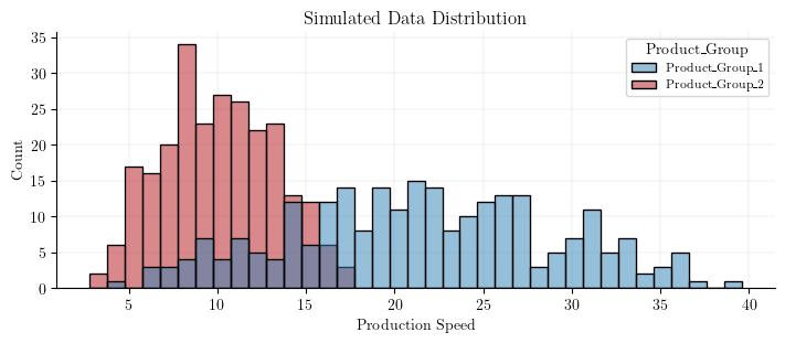
To illustrate the power of hierarchical regression in handling missing data, let’s consider a simulated example from a manufacturing context. We’ll analyze how different machine process parameters affect the production speed between two products groups.
In this simulation, we generate data for two product groups with different dependencies on machine process parameters:
Product Group 1 depends on feed speed and pull acceleration.
Product Group 2 depends on feed speed, pull acceleration, and cutting wait time.
Crucially, the cutting wait time for Product Group 1 is set to NaN, simulating a scenario where this parameter is not applicable or measured for this group.
Code
import matplotlib.pyplot as pltimport numpy as npimport numpyroimport pandas as pdimport seaborn as snsimport jax.numpy as jnpimport numpyro.distributions as distfrom jax import randomfrom numpyro.infer import Predictiveplt.style.use("https://raw.githubusercontent.com/GStechschulte/filterjax/main/docs/styles.mplstyle")
n_samples =500# Generate machine process parameters for both groupsfeed_speed = np.random.uniform(1, 10, n_samples)pull_acceleration = np.random.uniform(0.5, 5, n_samples)cutting_wait_time = np.random.uniform(0.1, 2, n_samples)# Create product groupsproduct_group = np.array(['Product_Group_1'] * (n_samples //2) + ['Product_Group_2'] * (n_samples //2))# Calculate production speedproduction_speed = np.zeros(n_samples)# Product Group 1: depends on feed speed and pull acceleration (Cutting Wait Time is NaN)mask_pg1 = product_group =='Product_Group_1'# Increased coefficients for Product Group 1 to ensure higher production speedproduction_speed[mask_pg1] = (feed_speed[mask_pg1] *2.5+ pull_acceleration[mask_pg1] *3+ np.random.normal(0, 0.5, sum(mask_pg1)))# Product Group 2: depends on all three parametersmask_pg2 = product_group =='Product_Group_2'production_speed[mask_pg2] = (feed_speed[mask_pg2] *1+ pull_acceleration[mask_pg2] *0.5+ cutting_wait_time[mask_pg2] *3+ np.random.normal(0, 0.5, sum(mask_pg2)))# Create DataFrame with NaN for Cutting Wait Time in Product Group 1simulated_dataset = pd.DataFrame({'Product_Group': product_group,'Feed_Speed': feed_speed,'Pull_Acceleration': pull_acceleration,'Cutting_Wait_Time': [np.nan if x =='Product_Group_1'else cutting_wait_time[i] for i,x inenumerate(product_group)],'Production_Speed': production_speed})
plt.figure(figsize=(7, 3))sns.histplot( data=simulated_dataset, x="Production_Speed", hue="Product_Group", binwidth=1)plt.xlabel("Production Speed")plt.title("Simulated Data Distribution");
To handle the missing data in our hierarchical model, we employ a technique called parameter masking. This approach allows us to effectively “turn off” certain parameters for specific groups where they are not applicable. Here’s how it works in our model:
Key aspects of this approach:
We use an indicators tensor to specify which parameters are relevant for each product group.
The input data X is masked to replace NaNs with zeros, and then multiplied by the indicators.
The weights w are also masked using the indicators, ensuring that irrelevant parameters don’t contribute to the predictions.
This approach allows the model to learn parameters even when data is missing for some groups, by effectively ignoring those parameters in the relevant calculations.
def model(indicators, config_idx, X, y=None): n_configs, n_params = indicators.shape# Create a masked version of X where NaNs are treated as zeros based on the indicators X_masked = jnp.where(jnp.isnan(X), 0.0, X) * indicators[config_idx]# Group-specific effectswith numpyro.plate("config_i", n_configs): alpha = numpyro.sample("alpha", dist.Normal(0., 5.))with numpyro.plate("param_i", n_params): w = numpyro.sample("w", dist.Normal(0., 5.))# Compute the weighted sum of features using indicators to zero-out unused parameters w_masked = jnp.multiply(w.T, indicators) eq = alpha[config_idx] + jnp.sum(jnp.multiply(X_masked, w_masked[config_idx]), axis=-1) mu = numpyro.deterministic("mu", eq) scale = numpyro.sample("scale", dist.HalfNormal(5.))with numpyro.plate("data", X.shape[0]): numpyro.sample("obs", dist.Normal(mu, scale), obs=y)
numpyro.render_model( model, model_args=( parameter_mask, config_idx, X, y ), render_params=True)
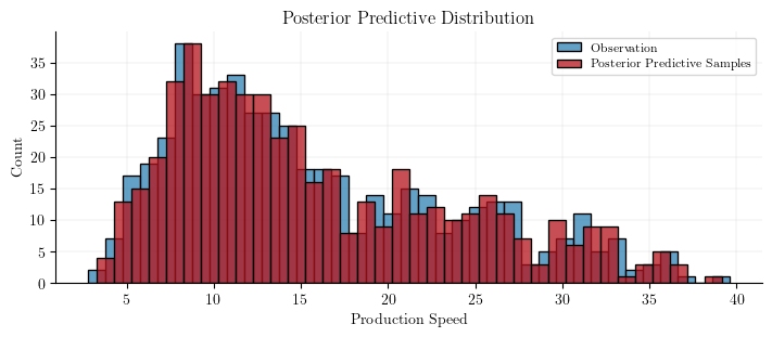
This summary shows us the estimated parameters, including group-specific intercepts (alpha) and weights for each parameter. Importantly, we’ll see that the weight for w[2,0] (cutting wait time) in Product Group 1 is effectively zero, as expected. We can now use the model to make predictions.
This plot compares the observed production speeds with the model’s predictions, allowing us to assess how well our model captures the underlying patterns in the data.
Hierarchical regression, combined with parameter masking, provides a powerful framework for analyzing grouped data with missing values. This approach allows us to:
Account for group-specific variations in the relationships between predictors and outcomes.
Handle missing data without requiring imputation or discarding incomplete cases.
Make predictions for new data, even when some predictors are not applicable to certain groups.
In real-world applications, such as manufacturing process modeling, this methodology enables more accurate modeling and prediction, leading to better decision-making and process improvements. By effectively leveraging all available data, including partial information from groups with missing predictors, we can gain deeper insights into complex processes.